ETC5510 Handout: Preparing for the course

The language of data analysis is the R programming language. It powers the work of people like data scientists, statisticians, social and natural scientists all over the world by allowing them to perform and communicate their data analyses in a principled way.

Throughout this course you’ll learn how to program in R and use the R programming language to make graphics, produce reports and even create interactive web applications. Before you do, you’ll need to get yourself ready by installing:

the R programming language on your computer
an integrated development environment (IDE) called RStudio that allows you to write R programs and interact with R code on your computer.

There are many other guides available for installing R that are just a web search away. One particular favourite is this guide by Kieran Healy from his Data Visualisation book. It is also worth reading the appendix which provides a comprehensive tutorial on how to read R documentation.

Getting started: what’s the difference?

You might be asking: so what’s the difference between R and RStudio? Julie Lowndes gives a great answer:

If R were an airplane, RStudio would be the airport, providing many, many supporting services that make it easier for you, the pilot, to take off and go to awesome places. Sure, you can fly an airplane without an airport, but having those runways and supporting infrastructure is a game-changer.

The following provides an overview of how to download, install and get up and running with R and RStudio.

Download and install R

You can download the R language from the Comprehensive R Archive Network or CRAN for short.

On the CRAN website, there are a list of links to download R for different operating systems, for example, Linux, (Mac) OS X and Windows. To download R to your computer, select the link that corresponds to your operating system. You can then install R.

Download and install RStudio

Once you have installed R, you are ready to install RStudio. For this course, the free version of RStudio is suitable. Get RStudio from the RStudio downloads page. Select the ‘Download’ link and then select the installer that corresponds to your operating system.

R and RStudio on Windows

If you are a Windows user, the CRAN website will redirect you to a page with a list of subdirectories. Select the link called base.

Please note, the following image is an example only; the version listed on the website may differ.

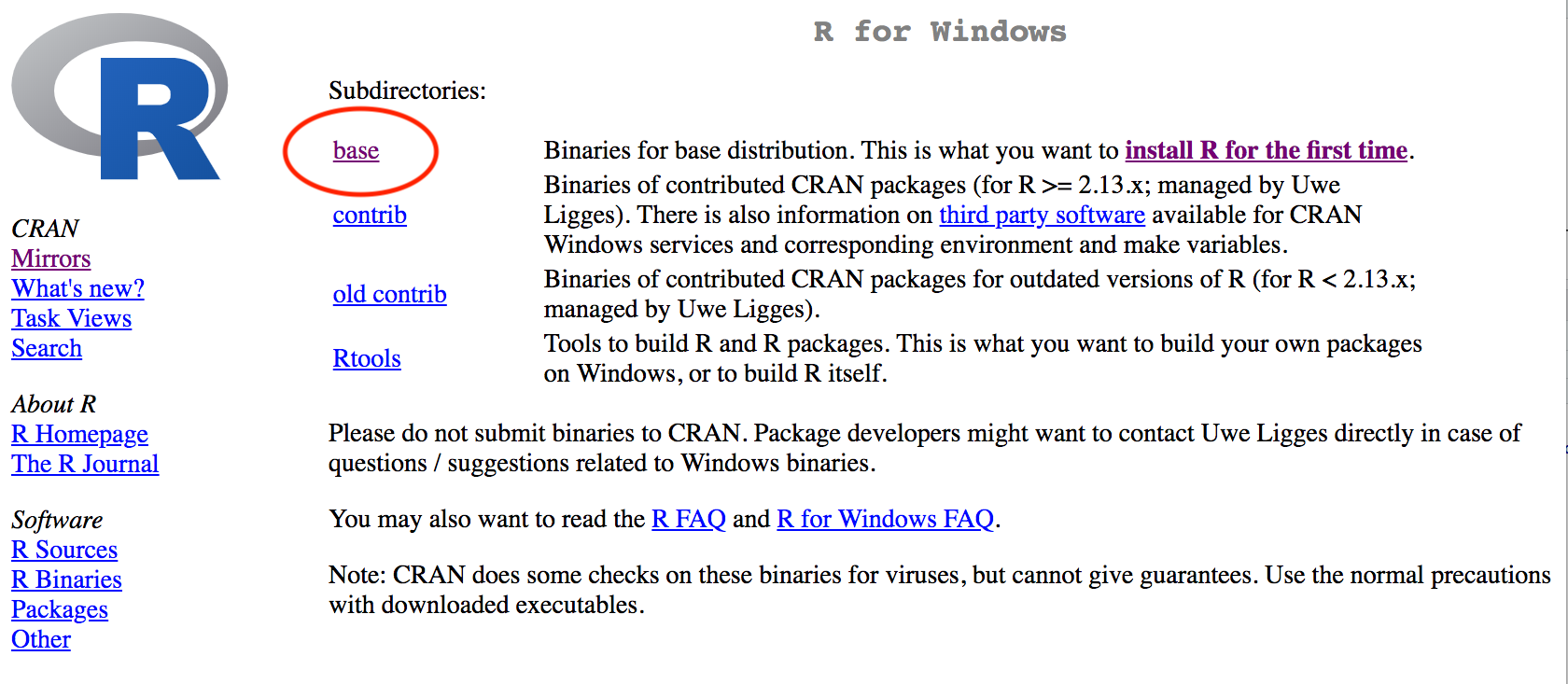
CRAN website, Windows link

You will be directed to a new page with a link to download R, for example, Download R 3.6.2 for Windows. Select the link to download R for Windows.

Once R has finished downloading, open the .exe file and work through the setup prompts. Once the setup is complete, download the latest version of the RStudio executable. Then, open the ‘.exe’ file and work through the setup prompts.

R and RStudio on Mac OS X

If you are a Mac OS X user, the CRAN website will redirect you to a page with a list of releases. Select the link, for example, R-3.6.2.pkg to download the latest release.

Please note, the following image is an example only; the version listed on the website may differ.

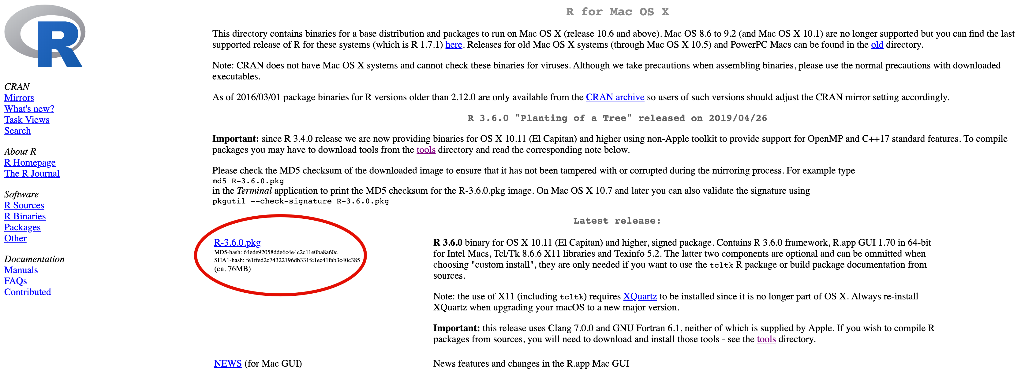
CRAN website, MacOS link

Once R has finished downloading, open the ‘.pkg’ and then work through the setup prompts. Once the setup is complete, download the latest version of RStudio. Then, open the ‘.dmg’ file and then follow the prompts.

Check your installation!

Well done, you’ve installed R and RStudio on your computer. Open RStudio to check that everything has installed correctly and to explore the RStudio interface. The RStudio interface should be divided into four panes:

scripts pane - the place where you write and save your R code.
tab for the console - the place where your code gets run. You can write code directly in here, but you might forget the code you write, so it’s a good idea to write your code in the scripts pane.
tab for Files, Plots, Packages, Help, and a Viewer - files are listed here, just like a ‘Finder’ in Mac OS X or ‘My Computer’ in Windows.
tab for Environment, History and Connections - things you create in R that are a result of code being run, such as data, objects and models are listed in the Environment.

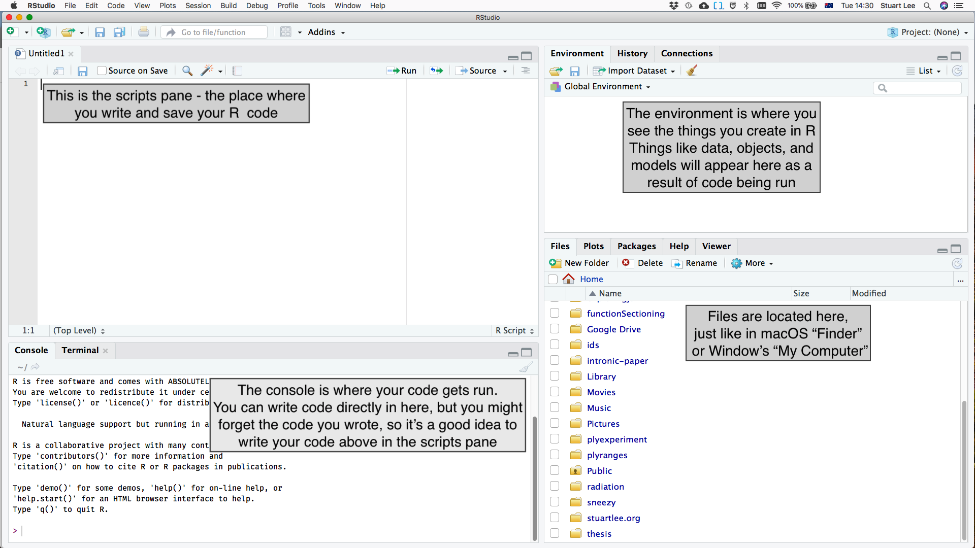
The Rstudio IDE

Playing with the console

Continue to explore RStudio by making your way through this exercise - using R as a calculator. At the prompt of your console in RStudio, run the following code chunk:

1999 * 2 / 1000

(39 + 13 + 2) / 4

cos(pi)

Store the results of your computation as an object using the left arrow <- (The shortcut in RStudio is Alt + -).

Again, at the prompt of your console in RStudio, run the following code chunk:

my_variable <- 7 * 8

What’s it doing?

This is read as my_variable gets the value of 7*8. In your RStudio the object called my_variable should be listed in the Environment pane.

Print the value of my_variable again by typing my_variable at the console.

Naming conventions are important!

Names of objects are important. You want them to be descriptive, and if you have multiple words in a name you need a way of dealing with that.

The convention we will use in this course is snake_case, where we separate multiple words by an underscore, and use all lower case. The most important thing though is to be consistent with your names.

Names are case sensitive and their spelling matters, otherwise R will not be able to correctly interpret the result.

Try running the following code:

my_Variable

my_varíable

Why does R give you an error?

R gives an error for the first line of code because there was an upper case V instead of a lower case v. Similarly, the second is an error because there was an accented i instead of an unaccented i.

Using functions

Most computations are performed by using functions. Functions take some input (arguments) and return an output. As an example, let’s use R’s built-in random number generator function runif() to generate 10 random numbers between 0 and 1.

If you type the number 10 as the first argument you will get 10 random numbers between 0 and 1.

runif(10)

#>  [1] 0.29614707 0.32769903 0.87429311 0.61414034 0.07141809 0.46152141
#>  [7] 0.19531762 0.09259858 0.12866640 0.01490003

If you type runif() in the RStudio console and then press TAB on your keyboard, a floating tooltip will appear that contains the names of the inputs to the function.

You can be more explicit by specifying each input:

runif(n = 10, min = 0, max = 1)

#>  [1] 0.4047332 0.5594455 0.2644337 0.2554977 0.2643289 0.7931630 0.3091934
#>  [8] 0.3777057 0.5361418 0.4788223

By changing the values of the arguments, we can finally generate our numbers between 0 and 10.

runif(10, min = 0, max = 10)

#>  [1] 3.247854 6.602838 5.587097 6.730972 9.619522 2.864200 4.059660 9.238728
#>  [9] 9.546601 3.739686

And you can save the result to an object using the <- operator.

y <- runif(10, min  = 0, max = 10)

y

#>  [1] 3.7441952 9.0954289 6.1879159 2.6384848 7.8668463 0.3675443 7.5540640
#>  [8] 3.2578185 5.9189878 6.2539780

Computing summaries

So far, you’ve explored the basics of using R as a calculator and creating objects and calling functions.

Consider expanding your R vocabulary by using the following functions to compute the mean using the mean() function, the variance using the var() function, and the range using the range() function of the object y you just created. Again, you can do this from the Console.

Remember, if you are not sure how to use the function, type the name of it in the console and press TAB on your keyboard.

Lab Exercise: so random!

You may have noticed the numbers you generated at your R console are different from the ones presented earlier. Why is that?
Look up the help file for the function set.seed by typing a question mark in front of it at the console: ?set.seed. If you need help understanding this read over this document.
How could you use it to ensure you get the same random numbers?

Setting up for success: data science workflow

When working on a new project, it is possible for your files to be spread out and stored in different locations across your computer.

This can create problems, particularly when you are programming because knowing exactly where your files are is really important. When they are spread out, this makes extra work for yourself.

Getting into the workflow

Storing files in folders, and folders in a ‘filing cabinet’ helps centralise your work: it keeps it organised so it is easier to find.

Using RStudio projects is like providing a filing cabinet for your work! Using them centralises your work, making your life easier as you do not have to manage where files are. For each project, you need to create one RStudio project.

Creating a new RStudio project

Make your way through the following steps to create an RStudio project on your computer for all the work that you’ll do in this course.

Step 1: Start a new project

On your computer, open RStudio. Then, select ‘File’ > ‘New Project’.

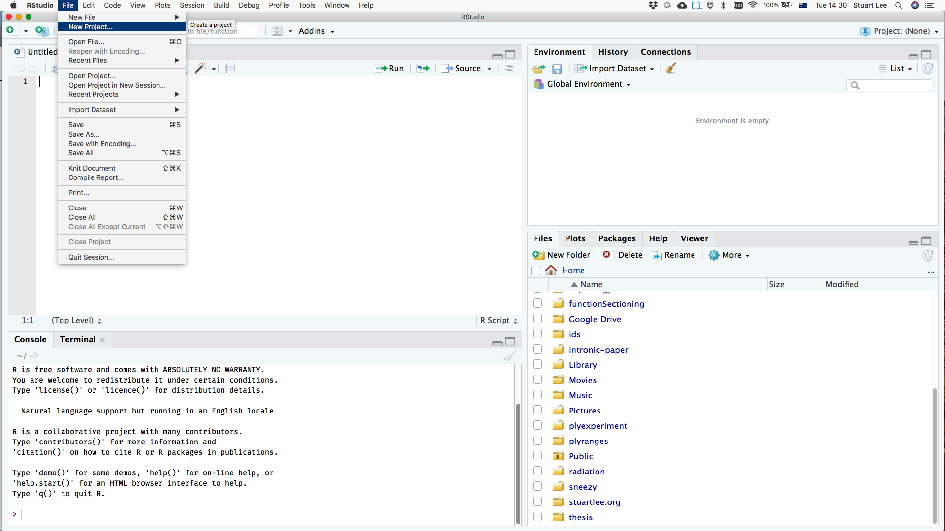
Setting up projects

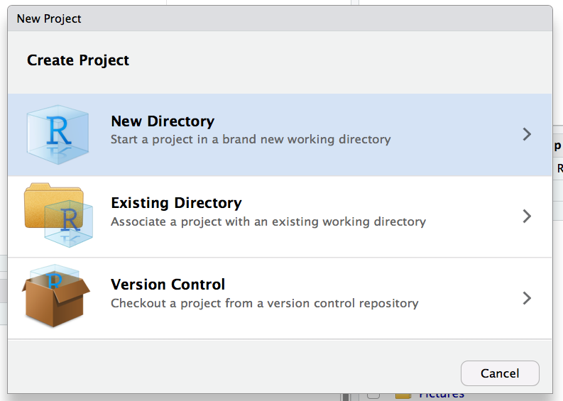
Step 2: Set a directory

A pop-up window labelled ‘New Project’ should be displayed in RStudio. From the pop-up window, select ‘New directory’.

Selecting a directory

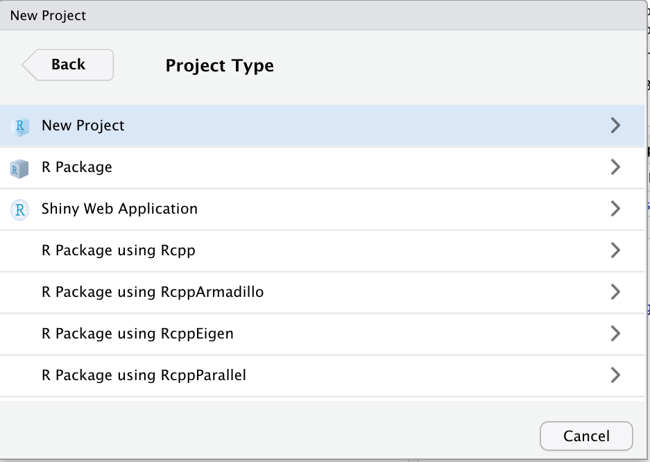
Step 3: Select the project type

You’re creating a new project, so select ‘New project’.

Project type

Step 4: Give your directory a name

Enter the name of the directory you want to create. It would be a good idea to name it by the course you are taking, like “intro_datascience”.

Select ‘Create project’ once you’ve named your directory.

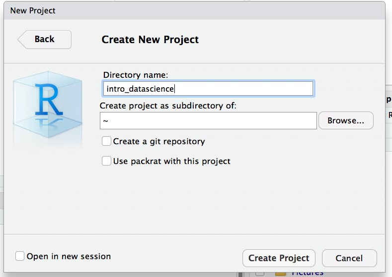
Naming the project

Step 5: Well done, you’ve now created a RStudio project!

Your RStudio will have a projects tab on the upper right hand corner. Remember, every time you start to work on something for this course, be sure to open this project!

Whenever you are ready to write code for the course go to your project folder and then select the ‘.Rproj’ file. This will automatically open RStudio and take you to the right directory!

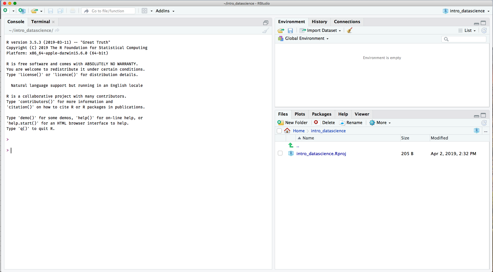
The final view:

Installing packages

Packages are the way R users share useful code. You can think of each R package as a book. Once you’ve installed a package, you can load the code contained in it using library - which is like checking out a book from the library!

There are more than 14,000 packages available on CRAN contributed by a range of R users, from experts to those relatively new to R. There are another thousand or so on the Bioconductor archive, which focuses primarily on bioinformatics applications. There are many more on people’s Github pages that may be in development. For example: Earo Wang’s mists package

As an example, you can install the rmarkdown package for making reproducible reports using the following code chunk:

install.packages("rmarkdown")

Lab Exercise: Setting yourself up for the course

Continue to develop your skills in RStudio by making your way through this exercise. Follow the instructions specified in ‘Creating a new RStudio project’ to create another RStudio project that will contain all your materials as you work through this course.

Then, use the console to install the tidyverse and visdat packages. You’ll use these packages throughout the course to read, visualise and analyse data.

After you’ve installed the packages, run library(tidyverse) at the console, then, run the following code chunk:

glimpse(diamonds)
filter(diamonds, carat <= 2.5)

What happened when you ran library(tidyverse) at the console?
Do you think that you’ll always need to run that code to use the tidyverse?
What happened when you ran the code chunk?